Prometheus Subquery Exploration
I’m still working my way through Prometheus: Up & Running, 2nd Edition, and now that I’ve reached Part 4 on PromQL, I decided it’s a good time to do a deeper dive into subqueries.
The documentation describes this feature as:
Subquery allows you to run an instant query for a given range and resolution. The result of a subquery is a range vector.
So what better way to fully grasp this feature than by breaking it down step by step?
Subqueries can seem a bit intimidating at first, but walking through them methodically not only helps demystify their structure, it also highlights just how powerful they can be when used effectively.
I’ll be using a single metric from Node Exporter and gradually work toward unraveling that subquery step by step. Starting simple helps keep things clear.
I’ll also be using the same evaluation time across all queries (2025-05-22 18:19:00).
First, let’s take a look at the Counter node_network_receive_bytes_total.
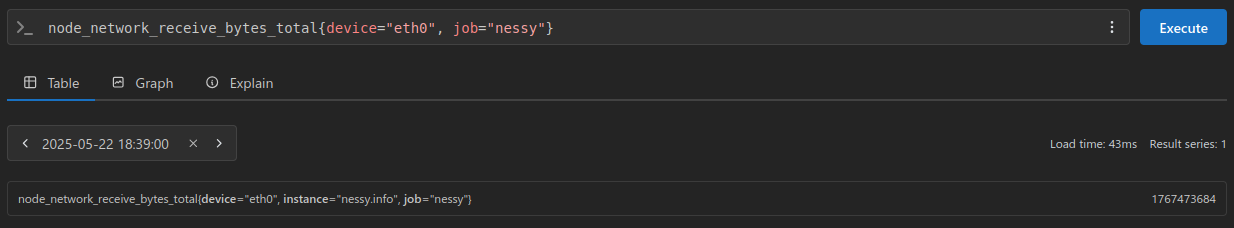
The result is an instant vector with the value 1767473684. This value represents the total number of bytes received since the exporter was first started.
Say we wanted not just the most recent value, but also values from the past:
By appending [5m] to the query, we can convert it into a range vector, allowing us to retrieve samples over the past 5 minutes.
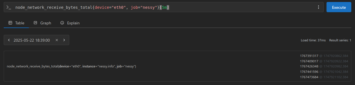
The results containing our Counter value paired with a Linux epoch timestamp for that sample:
1767391317 @ 1747920862.384
1767409017 @ 1747920922.384
1767426348 @ 1747920982.384
1767441596 @ 1747921042.384
1767473684 @ 1747921102.384
Notice the bottom value being the same as when we queried for the instant vector above.
To quickly get a friendly timestamp use your handy date command:
$ date -d @1747921102.384
Thu May 22 08:38:22 AM CDT 2025
As we know, ranged results like this should be observed using the rate() function, which gives us the value 343.1958333333333 (bytes per second):
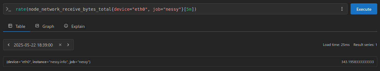
With a bit of math we can take the most recent counter value, subtract if from the oldest, then divide that by our observation window (minus one as edge bound apply) to see roughly what rate() is doing under the hood:
>>> (1767473684 - 1767391317) / (60 * 4)
343.1958333333333
With that out of the way, lets look at a subquery.
To keep things straightforward, my subquery will use [1m:1m], a 1-minute range with a 1-minute resolution.
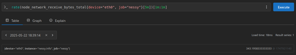
Notice that the result value is identical to when we didn’t use a subquery (however, it does contain a timestamp as it is a range vector).
That’s because, at this range and resolution, we’re effectively just asking for the latest data point, which results in the same outcome as querying without the subquery.
Now, let’s unlock the true power of subqueries by asking for a longer range, lets say the last five minutes:
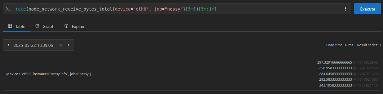
With a longer range we receive back 5 samples, each the rate() at that time.
And our most recent result matches our expected value of 343.1958333333333:
297.32916666666665 @ 1747920900
258.9583333333333 @ 1747920960
284.6458333333333 @ 1747921020
292.5833333333333 @ 1747921080
343.1958333333333 @ 1747921140
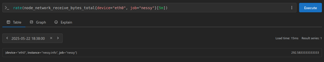
We can confirm these by changing our evaluation window back 1 minute (from 18:39:00 to 18:38:00) and we’d expect the same value as the above list’s second to the bottom value: 292.5833333333333
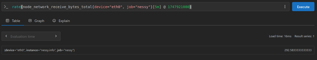
We could have also used the @ notation to specify the timestamp (the one paired with our 292.5833333333333 value) within the query:
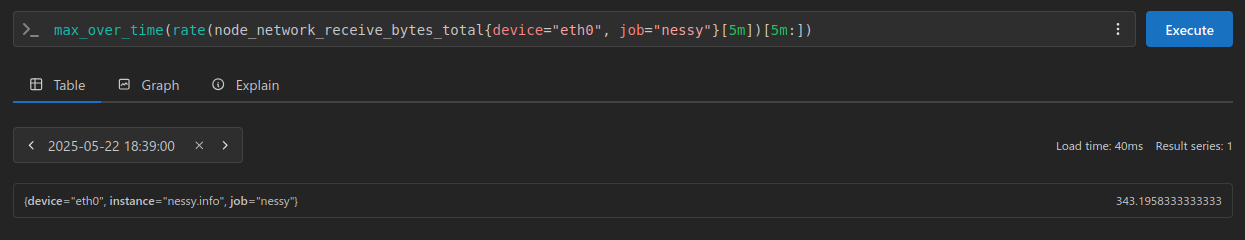
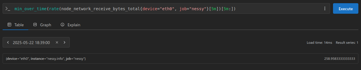
A couple functions that will be common with subqueries is to get the observed max_over_time or min_over_time values from these ranges.
Our max value being 343.1958333333333, and min being 258.9583333333333:
Finally, let’s wrap things up by comparing a graph without a subquery to see how the results visualize.
This graph utilizes the same evaluation window and displays the last 5 minutes:
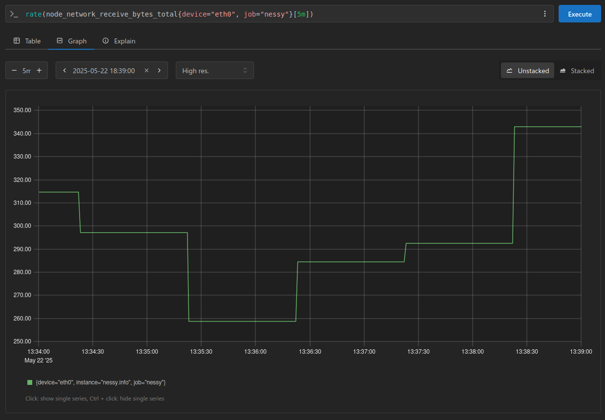
As you can see, the most recent 5 steps align perfectly with our observations and values posted above.