Understanding Quartiles Using Python
I’m continuing my journey through Prometheus: Up & Running, 2nd Edition and I’ve just wrapped up Chapter 14, which covered Aggregation Operators. In the chapter, we briefly explore stddev (Standard Deviation) and the quantile functions. As with previous chapters, I’m taking this as an opportunity to dive deeper into these concepts and use python to break it down.
Like my previous post, I’ll begin by pulling samples from Prometheus.
The Data
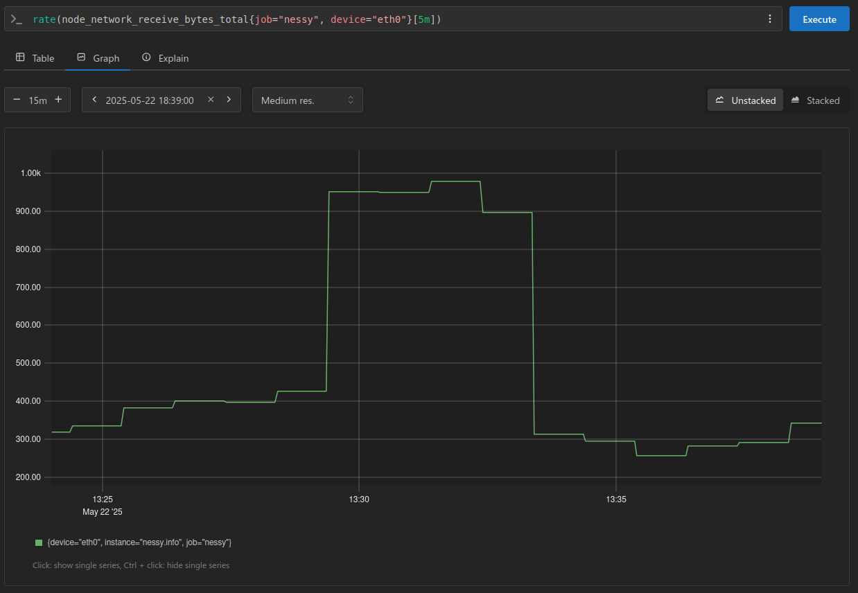
I’ll continue using the node_network_receive_bytes_total metric to illustrate the concepts, looking at the rate() of bytes received over a 15 minute window:
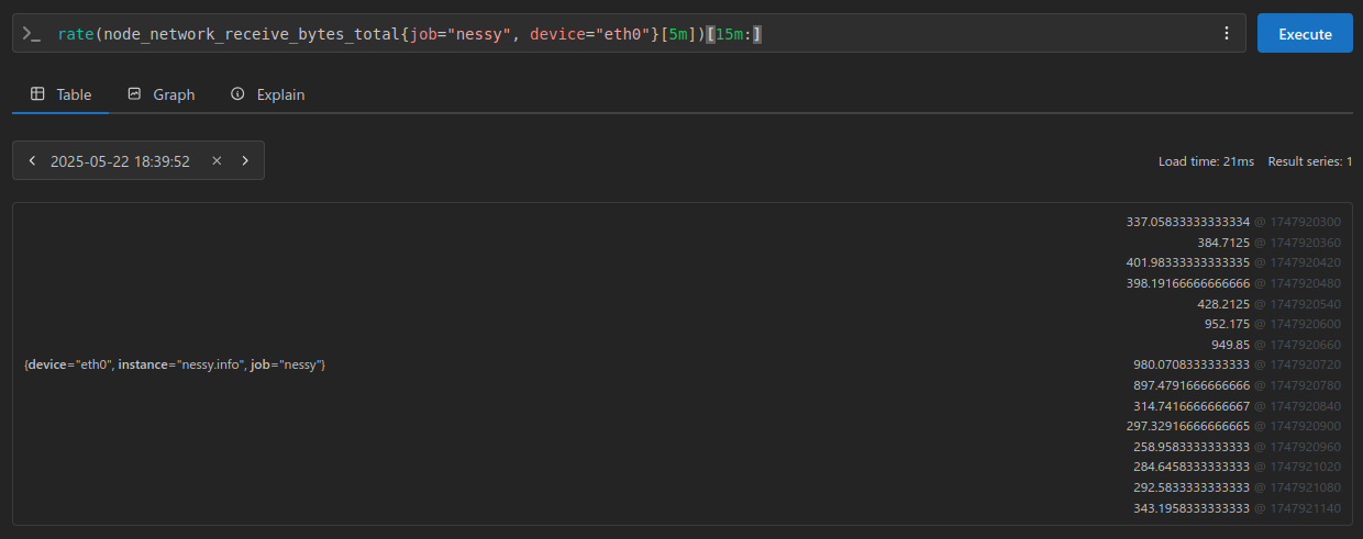
From the above PromQL I’ve extracted the samples and stored them:
>>> samples = [
...     337.05833333333334,
...     384.7125,
...     401.98333333333335,
...     398.19166666666666,
...     428.2125,
...     952.175,
...     949.85,
...     980.0708333333333,
...     897.4791666666666,
...     314.7416666666667,
...     297.32916666666665,
...     258.9583333333333,
...     284.6458333333333,
...     292.5833333333333,
...     343.1958333333333
... ]
Using these samples I’ll go ahead and get their standard deviation and average from Prometheus:
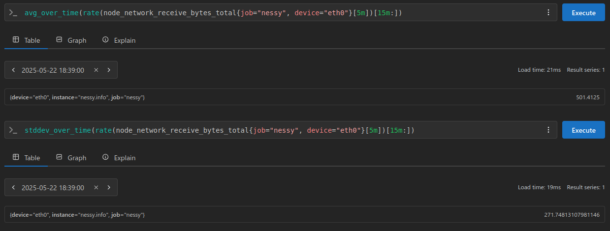
In the above calculations we receive the following results:
average / mean     = 501.4125
standard deviation = 271.74813107981146
Lets go ahead and see if we can produce the same outcomes using python.
I want to keep things simple, and without using any helper libraries that blurs the math or algorithms:
>>> avg = sum(samples) / len(samples)
>>>
>>> print(avg)
501.4125
>>> stddev = (sum([(i - avg) ** 2 for i in samples]) / len(samples)) ** .5
>>>
>>> print(stddev)
271.7481310798114
Great, those seem to compare to Prometheus nicely.
Quartiles - using a mean based approach
if you assume your data is normally distributed, you can approximate the quartiles using the mean and standard deviation.
>>> Q1 = avg - stddev
>>> Q2 = avg
>>> Q3 = avg + stddev
>>>
>>> print(f'Q1: {Q1}\nQ2: {Q2}\nQ3: {Q3}')
Q1: 229.66436892018862
Q2: 501.4125
Q3: 773.1606310798114
The Interquartile Range - when using mean based Quartiles
The interquartile range (IQR) is a measure of statistical dispersion, specifically the range between the first quartile (Q1) and the third quartile (Q3) of a dataset.
>>> IQR = Q3 - Q1
>>>
>>> print(IQR)
543.4962621596228
Outlier Detection:
The IQR can be used to identify outliers by defining boundaries based on Q1 - 1.5 * IQR and Q3 + 1.5 * IQR.
>>> lower_outlier_threshold = Q1 - 1.5 * IQR
>>> upper_outlier_threshold = Q3 + 1.5 * IQR
>>>
>>> print(f'lower: {lower_outlier_threshold}')
>>> print(f'upper: {upper_outlier_threshold}')
lower: -585.5800243192456
upper: 1588.4050243192455
With these values, you could easily iterate through the samples to identify any potential outliers:
>>> for sample in samples:
...     if sample > upper_outlier_threshold:
...         print(f'{sample} appear to be an upper anomaly')
...     elif sample < lower_outlier_threshold:
...         print(f'{sample} appear to be a lower anomaly')
...     else:
...         print(f'  no anomaly detected for {sample}')
  no anomaly detected for 337.05833333333334
  no anomaly detected for 384.7125
  no anomaly detected for 401.98333333333335
  no anomaly detected for 398.19166666666666
  no anomaly detected for 428.2125
  no anomaly detected for 952.175
  no anomaly detected for 949.85
  no anomaly detected for 11980.070833333333
  no anomaly detected for 897.4791666666666
  no anomaly detected for 314.7416666666667
  no anomaly detected for 297.32916666666665
  no anomaly detected for 258.9583333333333
  no anomaly detected for 284.6458333333333
  no anomaly detected for 292.5833333333333
  no anomaly detected for 343.1958333333333
One challenge with outlier detection when relying on the mean is that averages can be misleading. To demonstrate this, let’s take a look at a similar example, this time, I’ll deliberately increase one sample to an unusually large value to highlight the impact:
>>> samples = [
...     337.05833333333334,
...     384.7125,
...     401.98333333333335,
...     398.19166666666666,
...     428.2125,
...     952.175,
...     949.85,
...     111980.0708333333333,  # anomaly
...     897.4791666666666,
...     314.7416666666667,
...     297.32916666666665,
...     258.9583333333333,
...     284.6458333333333,
...     292.5833333333333,
...     343.1958333333333
... ]
Lets use the same process as before to calculate average/mean and standard deviations:
>>> Q1 = avg - stddev
>>> Q2 = avg
>>> Q3 = avg + stddev
>>>
>>> print(f' Q1: {Q1}\n Q2: {Q2}\n Q3: {Q3}')
Q1: -19915.812206646755
Q2: 7901.4125
Q3: 35718.63720664675
Notice how that single outlier is really pushing all our quartiles?
You’ll also notice that our interquartile range (IQR) is significantly higher than the majority of our samples.
>>> IQR = Q3 - Q1
>>>
>>> print(IQR)
55634.44941329351
And due to that our thresholds are outrageous:
>>> lower_outlier_threshold = Q1 - 1.5 * IQR
>>> upper_outlier_threshold = Q3 + 1.5 * IQR
>>>
>>> print(f'lower: {lower_outlier_threshold}')
>>> print(f'upper: {upper_outlier_threshold}')
lower: -103367.48632658701
upper: 119170.31132658702
Using our simple anomaly checker, still nothing is detected:
>>> for sample in samples:
...     if sample > upper_outlier_threshold:
...         print(f'{sample} appear to be an upper anomaly')
...     elif sample < lower_outlier_threshold:
...         print(f'{sample} appear to be a lower anomaly')
...     else:
...         print(f'  no anomaly detected for {sample}')
  no anomaly detected for 337.05833333333334
  no anomaly detected for 384.7125
  no anomaly detected for 401.98333333333335
  no anomaly detected for 398.19166666666666
  no anomaly detected for 428.2125
  no anomaly detected for 952.175
  no anomaly detected for 949.85
  no anomaly detected for 111980.07083333333
  no anomaly detected for 897.4791666666666
  no anomaly detected for 314.7416666666667
  no anomaly detected for 297.32916666666665
  no anomaly detected for 258.9583333333333
  no anomaly detected for 284.6458333333333
  no anomaly detected for 292.5833333333333
  no anomaly detected for 343.1958333333333
This is where a median Quartile approach is ideal (because our dataset is not very uniform with that outlier).
Quartiles - using a median based approach
To find quartiles using the median method, first arrange the data in ascending order. Then, identify the median (Q2), which divides the data into two halves. The lower quartile (Q1) is the median of the lower half of the data, and the upper quartile (Q3) is the median of the upper half.
If the set has an odd number of elements, the median is the middle element. If the set has an even number of elements, the median is the average of the two middle elements
So lets write a bit of basic python to break it down:
>>> sorted_samples = sorted(samples)
>>> sample_count = len(sorted_samples)
>>>
>>> print(f'sorted_samples: \n{sorted_samples}\n')
sorted_samples:
[
  258.9583333333333,
  284.6458333333333,
  292.5833333333333,
  297.32916666666665,
  314.7416666666667,
  337.05833333333334,
  343.1958333333333,
  384.7125,
  398.19166666666666,
  401.98333333333335,
  428.2125,
  897.4791666666666,
  949.85,
  952.175,
  11980.070833333333
 ]
Now that our samples are sorted we need to check if the list is even or odd, to do this a simple modulo division will work:
>>> if sample_count % 2:
...     Q2 = sorted_samples[sample_count // 2]
... else:
...     # in case of even take the center edge numbers and
...     # get their average
...     lower_edge = sorted_samples[(sample_count // 2) - 1]
...     upper_edge = sorted_samples[(sample_count // 2)]
...     Q2 = (lower_edge + upper_edge) / 2
...
... print(f'Q2: {Q2})
Q2: 384.7125
Next we will need to determine our median value within the upper and lower halves of our samples. Normally this would be done in the loop above, but I’m breaking it up to explain step by step:
>>> if sample_count % 2:
...     lower_set = sorted_samples[:sample_count // 2]
...     upper_set = sorted_samples[(sample_count // 2) + 1:]
...     print(f'lower: {lower_set}')
...     print(f'upper: {upper_set}')
...     Q1 = lower_set[len(lower_set) // 2]
...     Q3 = upper_set[len(upper_set) // 2]
... else:
...     lower_set = sorted_samples[:sample_count // 2]
...     upper_set = sorted_samples[(sample_count // 2):]
...     print(f'lower: {lower_set}')
...     print(f'upper: {upper_set}')
...     Q1 = lower_set[len(lower_set) // 2]
...     Q3 = upper_set[len(upper_set) // 2]
...
... print(f'Q1: {Q1}')
... print(f'Q2: {Q2}')
... print(f'Q3: {Q3}')
lower: [
  258.9583333333333,
  284.6458333333333,
  292.5833333333333,
  297.32916666666665,   # median
  314.7416666666667,
  337.05833333333334,
  343.1958333333333
]

upper: [
  398.19166666666666,
  401.98333333333335,
  428.2125,
  897.4791666666666,   # median
  949.85,
  952.175,
  11980.070833333333
]

Q1: 297.32916666666665
Q2: 384.7125
Q3: 897.4791666666666
The Interquartile Range - when using median based Quartiles
>>> IQR = Q3 - Q1
>>>
>>> print(f'IQR: {IQR}\n')
IQR: 600.15
Notice how our interquartile range is no longer as greatly effected by our single outlier.
Outlier Detection:
>>> lower_outlier_threshold = Q1 - 1.5 * IQR
>>> upper_outlier_threshold = Q3 + 1.5 * IQR
>>>
>>> print(f'lower: {lower_outlier_threshold}')
>>> print(f'upper: {upper_outlier_threshold}')
lower: -602.8958333333333
upper: 1797.7041666666664
With this approach we should be able to capture that single anomaly:
>>> for sample in samples:
...     if sample > upper_outlier_threshold:
...         print(f'{sample} appear to be an upper anomaly')
...     elif sample < lower_outlier_threshold:
...         print(f'{sample} appear to be a lower anomaly')
...     else:
...         print(f'  no anomaly detected for {sample}')
 no anomaly detected for 337.05833333333334
  no anomaly detected for 384.7125
  no anomaly detected for 401.98333333333335
  no anomaly detected for 398.19166666666666
  no anomaly detected for 428.2125
  no anomaly detected for 952.175
  no anomaly detected for 949.85
111980.07083333333 appear to be an upper anomaly
  no anomaly detected for 897.4791666666666
  no anomaly detected for 314.7416666666667
  no anomaly detected for 297.32916666666665
  no anomaly detected for 258.9583333333333
  no anomaly detected for 284.6458333333333
  no anomaly detected for 292.5833333333333
  no anomaly detected for 343.1958333333333
Quartile Buckets
Now that we have our Q1, Q2, Q3 values, we can store counts of our samples in their appropriate bucket:
>>> def get_quartiles(samples: list):
...   """
...   Returns samples with in their quartile buckets
...   """
...
...   print(f'Samples:\n {samples}\n')
...   print(f'Quartiles:\n Q1 = {Q1}\n Q2 = {Q2}\n Q3 = {Q3}\n')
...
...   first_bucket = f'-∞ - {int(Q1)}'
...   second_bucket = f'{int(Q1)} - {int(Q2)}'
...   third_bucket = f'{int(Q2)} - {int(Q3)}'
...   fourth_bucket = f'{int(Q3)} - ∞'
...
...   quartiles = {
...     first_bucket: 0,
...     second_bucket: 0,
...     third_bucket: 0,
...     fourth_bucket: 0
...   }
...
...   for sample in samples:
...
...     if sample < Q1:
...       quartiles[first_bucket] += 1
...
...     elif sample > Q3:
...       quartiles[fourth_bucket] += 1
...
...     elif sample <= Q2:
...       quartiles[second_bucket] += 1
...
...     elif sample >= Q2:
...       quartiles[third_bucket] += 1
...
...   return quartiles
...
... quartiles = get_quartiles(samples)
... print('\nBuckets:')
... print(quartiles)
Samples: [
337.05833333333334,
384.7125,
401.98333333333335,
398.19166666666666,
428.2125,
952.175,
949.85,
11980.070833333333,
897.4791666666666,
314.7416666666667,
297.32916666666665,
258.9583333333333,
284.6458333333333,
292.5833333333333,
343.1958333333333
]
Quartiles:
Q1 = 297.32916666666665
Q2 = 384.7125
Q3 = 897.4791666666666
Buckets:
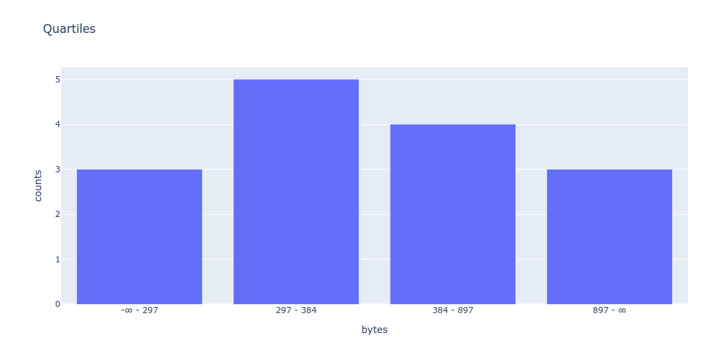
{'-∞ - 297': 3, '297 - 384': 5, '384 - 897': 4, '897 - ∞': 3}
In theory, we could plot our own graph directly from Python. (Of course, you’ll need to have pandas, numpy, and plotly installed.)
>>> import pandas as pd
...
... df = pd.DataFrame(quartiles, index=['counts'])
... print(df.T)
           counts
-∞ - 297        3
297 - 384       5
384 - 897       4
897 - ∞         3
And the plot
>>> import plotly.express as px
... import plotly.io as pio
... pio.renderers.default = 'iframe'
...
... fig = px.bar(df.T, title="Quartiles")
... fig.update_layout(xaxis_title="bytes", yaxis_title="counts")
... fig.show()
This is all great for understanding the fundamentals, but in practice we would be using Prometheus, and probably the quantile_over_time function:
NOTE: we are back to using our non anomaly injected dataset here
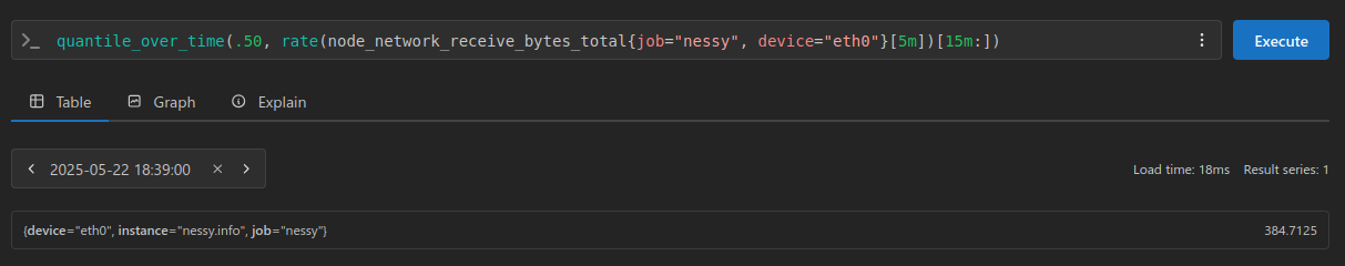
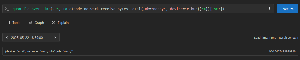
The result here being 384.7125 for our 0.50 quantile (or 50th percentile), and 960.5437499999998 for our 0.95 quantile. (or 95th percentile)
And lastly for graphing we would be using something like a Grafana histogram visualization:
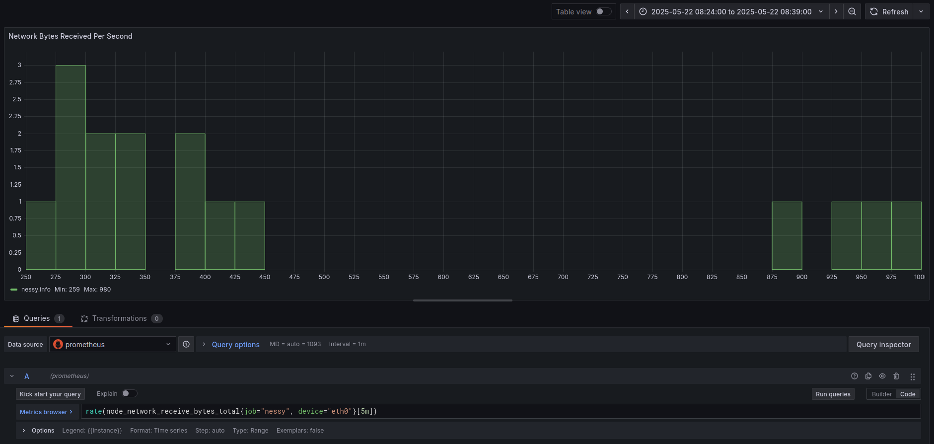
Cheers, and happy hacking!