Prometheus and the Deriv Function
As I wrap up Prometheus: Up & Running, 2nd Edition, I wanted to take one last deep dive into the math behind one of Prometheus’s functions: deriv().
The documentation says:
deriv(v range-vector) calculates the per-second derivative of each float time series in the range vector v, using simple linear regression.
And according to Prometheus: Up & Running:
The deriv function uses least-squares regression to estimate the slope of each of the time series in a range vector.
Data
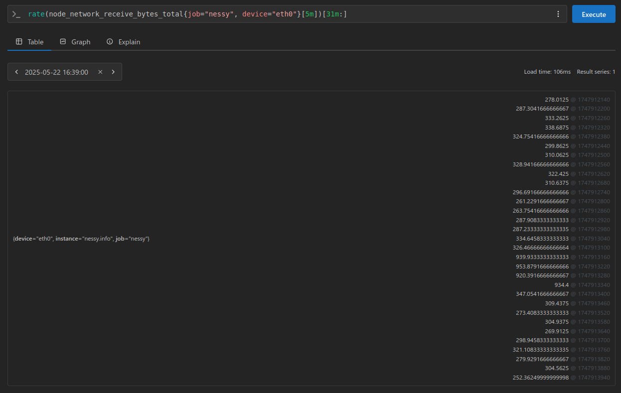
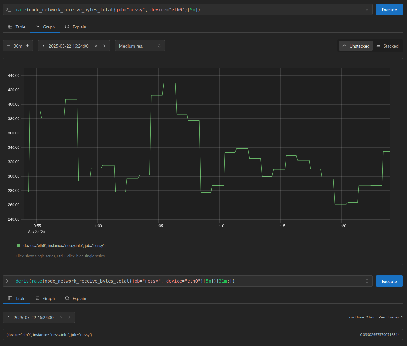
Just like last time, let’s take a few samples from Prometheus for the node_network_receive_bytes_total metric:
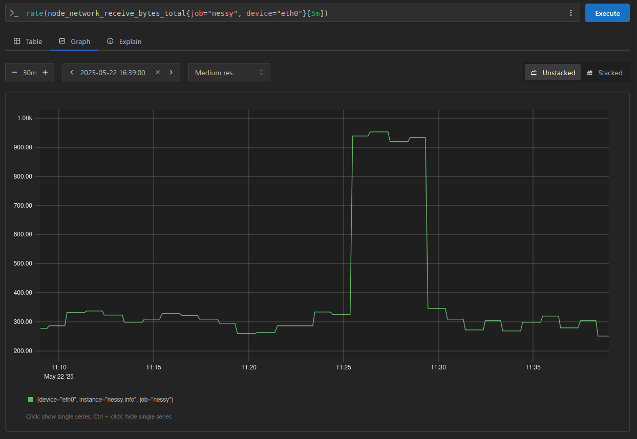
The graph above visualizes network bytes received per second over a 30-minute window. With a scrape interval of 1 minute, we can expect 30 data points, plus one additional sample to account for the window boundary.
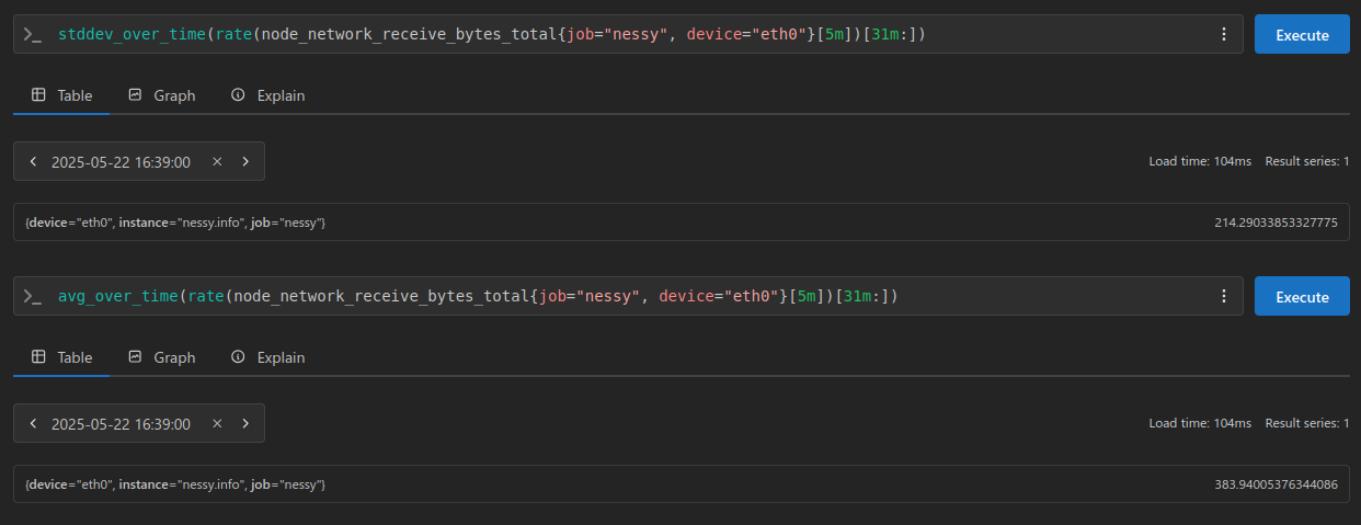
Using these samples, I also calculated the average and standard deviation for reference. This helps me verify that my inputs and calculations align correctly when I process the data in Python.
Now, let’s take a closer look at the deriv function, and examine the results it produces.
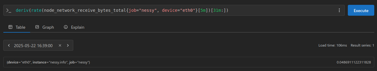
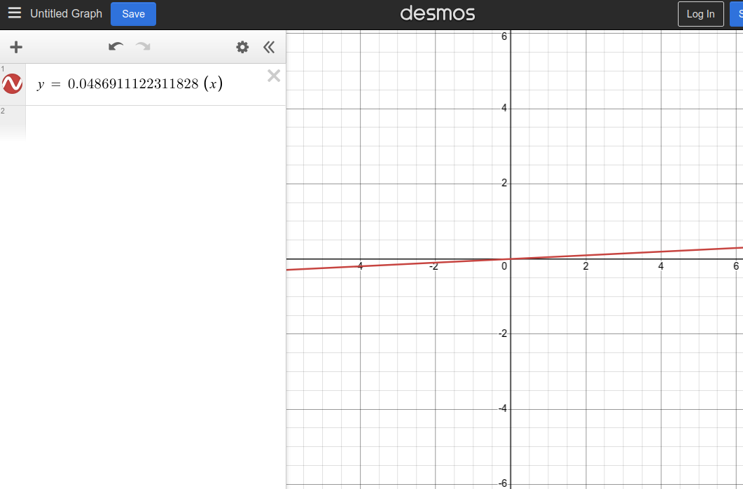
A value of 0.0486911122311828 here is our range vector’s slope using Least Square Method Formula.
So, what does the slope look like? We can easily visualize it by plugging the data into a Desmos an online graphing calculator:
The formula
y = mxrepresents a linear equation whereyandxare variables, andmis a constant representing the slope or gradient of a line
The Math
Let’s take it a step further by implementing the Least Squares Method in Python manually.
I find that working through it this way helps solidify our understanding of the underlying concepts.
Slope (m) Formula: m = n(∑xy)−(∑x)(∑y) / n(∑x2)−(∑x)2
Intercept (c) Formula: c = (∑y)−a(∑x) / n
In Python lets process our points Prometheus gave us:
>>> raw = '''278.0125 @ 1747912140
... 287.3041666666667 @ 1747912200
... 333.2625 @ 1747912260
... 338.6875 @ 1747912320
... 324.75416666666666 @ 1747912380
... 299.8625 @ 1747912440
... 310.0625 @ 1747912500
... 328.94166666666666 @ 1747912560
... 322.425 @ 1747912620
... 310.6375 @ 1747912680
... 296.69166666666666 @ 1747912740
... 261.2291666666667 @ 1747912800
... 263.75416666666666 @ 1747912860
... 287.9083333333333 @ 1747912920
... 287.23333333333335 @ 1747912980
... 334.6458333333333 @ 1747913040
... 326.46666666666664 @ 1747913100
... 939.9333333333333 @ 1747913160
... 953.8791666666666 @ 1747913220
... 920.3916666666667 @ 1747913280
... 934.4 @ 1747913340
... 347.0541666666667 @ 1747913400
... 309.4375 @ 1747913460
... 273.4083333333333 @ 1747913520
... 304.9375 @ 1747913580
... 269.9125 @ 1747913640
... 298.9458333333333 @ 1747913700
... 321.10833333333335 @ 1747913760
... 279.9291666666667 @ 1747913820
... 304.5625 @ 1747913880
... 252.36249999999998 @ 1747913940'''
...
... samples = [ float(i.split()[0]) for i in raw.split('\n') ]
...
... print(f'{len(samples)}')
31 samples:
And to make sure we are aligned with Prometheus we can quickly get our average and standard deviation (something I covered in my last post Understanding Quartiles Using Python):
>>> avg = sum(samples) / len(samples)
... print(avg)
383.94005376344086
>>> stddev = (sum([(i - avg) ** 2 for i in samples]) / len(samples)) ** .5
... print(stddev)
214.29033853327775
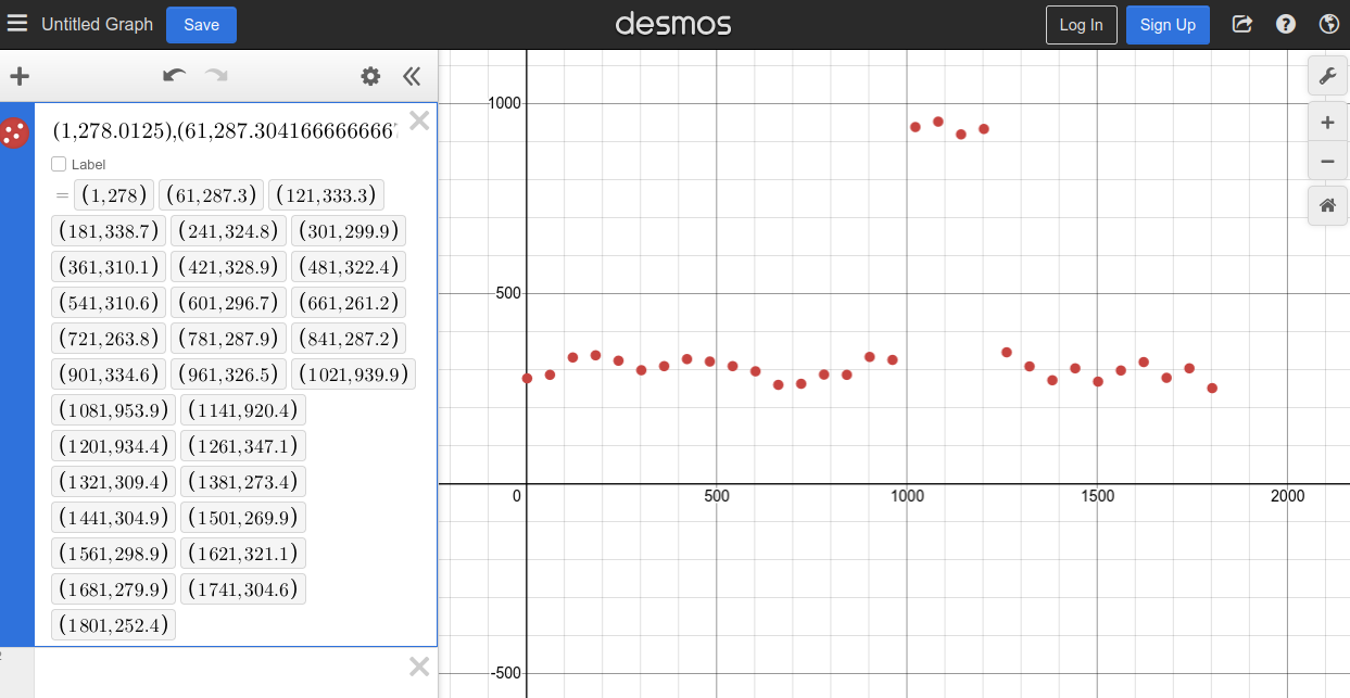
Instead of extracting timestamps, I’ll simplify things by starting our points at 1 and incrementing them by 60 seconds for each iteration. This approach makes it easy to plug the results directly into Desmos:
>>> # x/y points for desmos graphing calc
... c = 1
... coords = []
... for s in samples:
...     coords.append((c, s))
...     c += 60
...
... print(coords)
[(1, 278.0125),
 (61, 287.3041666666667),
 (121, 333.2625),
 (181, 338.6875),
 (241, 324.75416666666666),
 (301, 299.8625),
 (361, 310.0625),
 (421, 328.94166666666666),
 (481, 322.425),
 (541, 310.6375),
 (601, 296.69166666666666),
 (661, 261.2291666666667),
 (721, 263.75416666666666),
 (781, 287.9083333333333),
 (841, 287.23333333333335),
 (901, 334.6458333333333),
 (961, 326.46666666666664),
 (1021, 939.9333333333333),
 (1081, 953.8791666666666),
 (1141, 920.3916666666667),
 (1201, 934.4),
 (1261, 347.0541666666667),
 (1321, 309.4375),
 (1381, 273.4083333333333),
 (1441, 304.9375),
 (1501, 269.9125),
 (1561, 298.9458333333333),
 (1621, 321.10833333333335),
 (1681, 279.9291666666667),
 (1741, 304.5625),
 (1801, 252.36249999999998)]
And there you have it, a scatter plot that perfectly matches our Prometheus graph:
Now, let’s write the Python code to implement the Least Squares Method:
>>> print(f'Number of Points: {len(coords)}\n')
...
... sum_xy = sum([ x * y for x, y in coords ])
... print(f'sum_xy: {sum_xy}')
...
... sum_x = sum([ x for x, _ in coords ])
... print(f'sum_x: {sum_x}')
...
... sum_y = sum([ y for _, y in coords])
... print(f'sum_y: {sum_y}')
...
... sum_x2 = sum([ x ** 2 for x, _ in coords ])
... print(f'sum_x2: {sum_x2}')
...
... print('------')
...
... print('\nSlope Equation:')
... print(f'({len(numbers)} * {sum_xy} - {sum_x} * {sum_y}) / ({len(numbers)} * {sum_x2} - {sum_x} ** 2)')
...
... top = len(numbers) * sum_xy - sum_x * sum_y
... bottom = len(numbers) * sum_x2 - sum_x ** 2
...
... slope = top / bottom
... print(f'\nSlope = {slope}')
...
... print('\nIntercept Equation:')
... print(f'({sum_y} - {slope} * {sum_x}) / {len(numbers)}')
...
... intercept = (sum_y - slope * sum_x) / len(numbers)
... print(f'\nIntercept = {intercept}')
Number of Points: 31

sum_xy: 11146641.75
sum_x: 27900
sum_y: 11902.141666666666
sum_x2: 34038000
------

Slope Equation:
(31 * 11146641.75 - 27900 * 11902.141666666666) / (31 * 34038000 - 27900 ** 2)

Slope = 0.0486911122311828

Intercept Equation:
(11902.141666666666 - 0.0486911122311828 * 27900) / 31

Intercept = 340.11805275537637
Notice how our slope matches Prometheus 🎉
With these results, we can plug them back into the equation and visualize how the line looks:
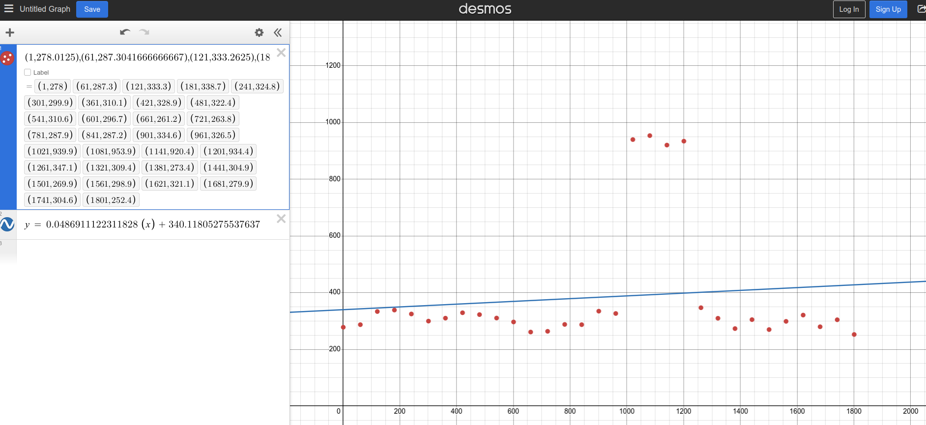
As we can see, the line isn’t a perfect fit for the data. This is due to the presence of outliers, which is one of the key limitations of the Least Squares Method:
The Least Squares method assumes that the data is evenly distributed and doesn’t contain any outliers for deriving a line of best fit. However, this method doesn’t provide accurate results for unevenly distributed data or data containing outliers.
Let’s see how the line and slope behave with a more uniform sample set:
Number of Points: 31

sum_xy: 8800330.870833334
sum_x: 27931
sum_y: 10114.370833333332
sum_x2: 34093831
------

Slope Equation:
(31 * 8800330.870833334 - 27931 * 10114.370833333332) / (31 * 34093831 - 27931 ** 2)

Slope = -0.035026573700716844

Intercept Equation:
(10114.370833333332 - -0.035026573700716844 * 27931) / 31

Intercept = 357.82896978606624
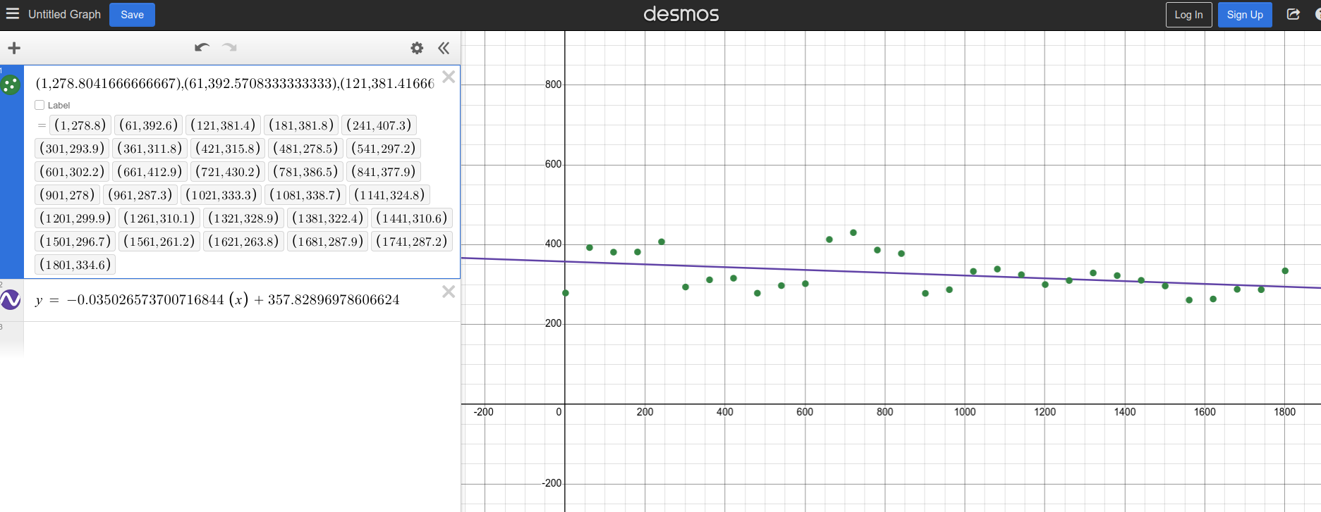
As we can clearly see, this line fits our sample much better.
That’s all for this post, hope you found it helpful!
Cheers, and happy hacking!